Credit Card Customer Segmentation

Numerical behaviour · customer profiles · anomaly exploration

Project: Unsupervised Machine Learning Workshop
Author: Gabriela Granja
Repository: GitHub
Documentation: GitHub Pages

Objective

This workshop uses unsupervised learning to explore behavioural patterns among credit-card customers without predefined segment labels. Because there is no ground-truth segmentation, model selection must combine internal clustering metrics with cluster balance and interpretable profiles in the original financial variables.

The resulting groups are segmentation hypotheses. They are not credit-risk decisions, fraud labels or recommendations for automated customer treatment.

Dataset

Item	Executed notebook result
Customers	8,950
Original columns	18
Behavioural variables after CUST_ID removal	17
Duplicate rows	0
Missing CREDIT_LIMIT values	1
Missing MINIMUM_PAYMENTS values	313

The numerical variables summarise six months of balance, purchase, cash-advance, payment, credit-limit, frequency and tenure behaviour. Their ranges differ substantially, and several monetary distributions are strongly right-skewed.

flowchart LR
    A[Inspect data] --> B[Impute medians]
    B --> C[Standardize]
    C --> D[PCA]
    D --> E[Select k]
    E --> F[Cluster]
    F --> G[Profile]
    G --> H[Detect anomalies]
    H --> I[Extend and test stability]

Data quality and preparation

CUST_ID is retained only for tracing records and excluded from modelling. The missing CREDIT_LIMIT and MINIMUM_PAYMENTS values are imputed with each column's median, a robust choice for the skewed monetary variables. No missing values remain after this step.

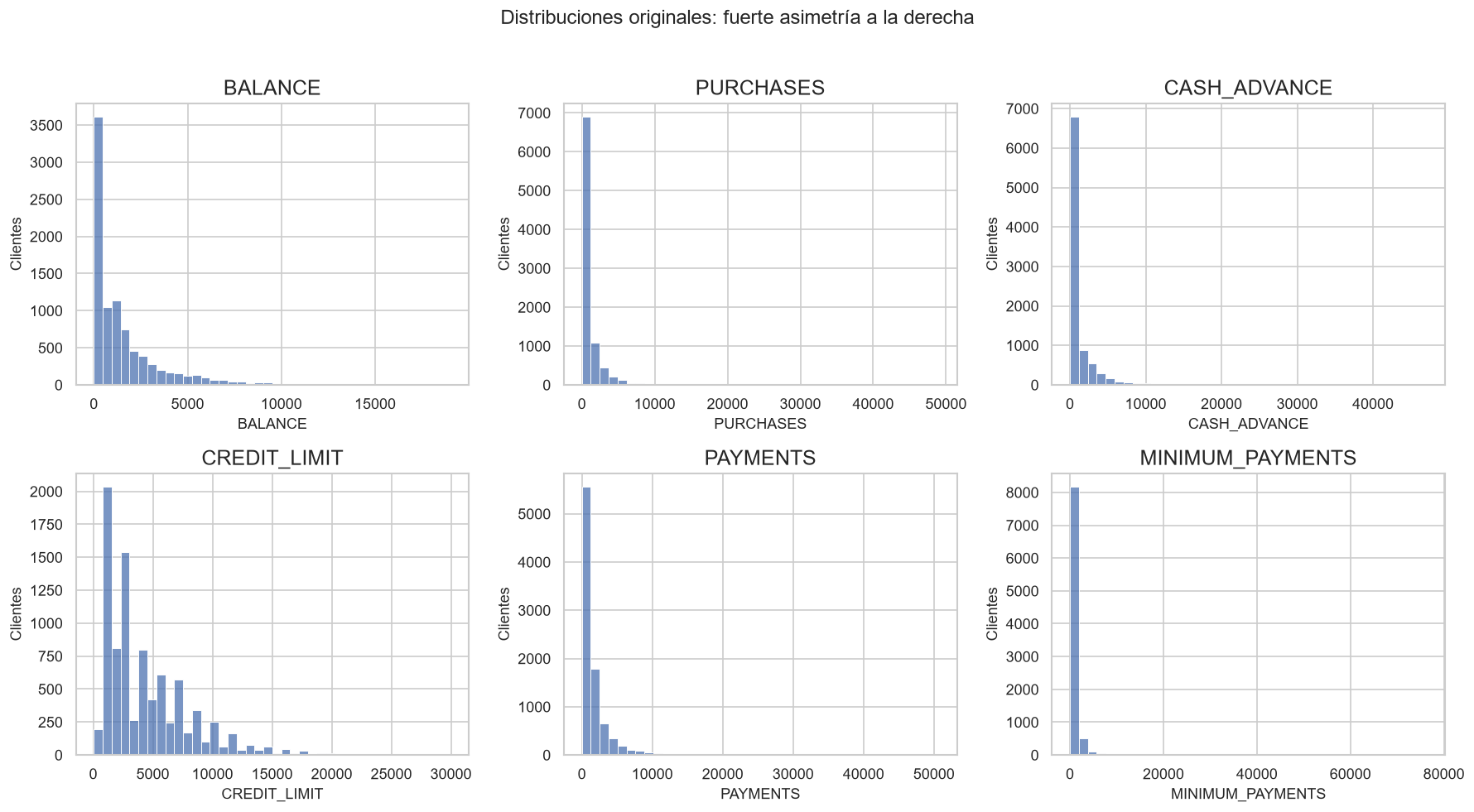
Figure 1. Six selected monetary and behavioural distributions from the executed baseline notebook.

The long right tails are visible rather than hidden: MINIMUM_PAYMENTS, PURCHASES, PAYMENTS and CASH_ADVANCE record skewness of 13.85, 8.14, 5.91 and 5.17 respectively. This motivates median imputation and cautions against interpreting raw means without context.

Feature scaling

All 17 modelling variables are transformed with StandardScaler. This prevents large monetary values from dominating Euclidean distances used by K-Means, hierarchical clustering and PCA. The executed check confirms approximately zero mean and unit standard deviation for every scaled feature.

PCA

PCA first quantifies how much of the standardized feature space can be retained in fewer dimensions.

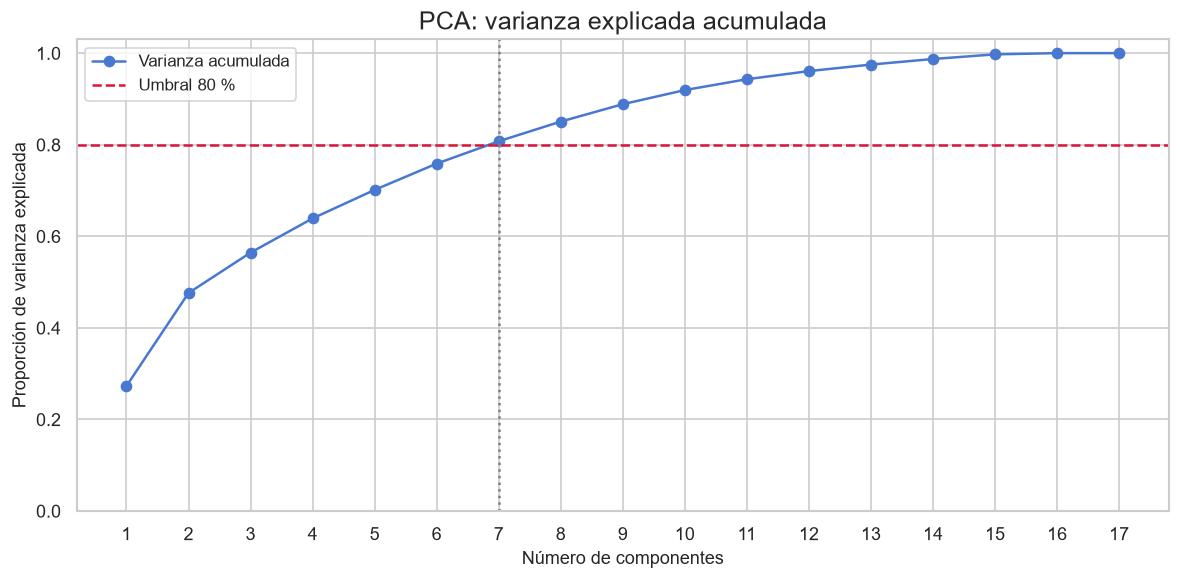
Figure 2. Cumulative explained variance across principal components; seven components retain 80.75%.

Seven components reach the selected 80% threshold, retaining 80.75% of the standardized variance. This is a compression result, not evidence of clusters.

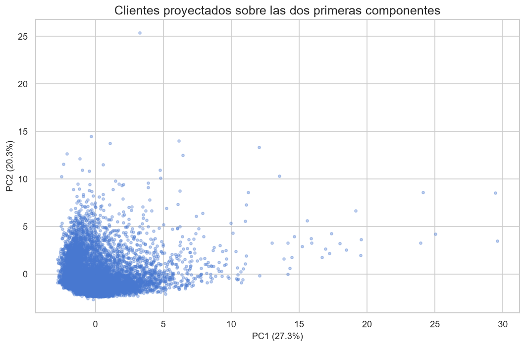
Figure 3. First two principal components, which together explain 47.61% of the standardized variance.

The two-dimensional view is useful for seeing the broad geometry but does not represent all original information. The continuous cloud offers no obvious visual ground truth, so clustering is evaluated in the complete standardized feature space unless stated otherwise.

K-Means model selection

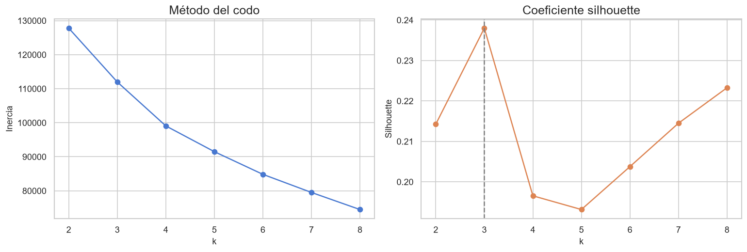
Figure 4. Inertia and sampled silhouette for k=2–8. The highest tested sampled silhouette selects k=3 at 0.238.

Inertia declines continuously, so the elbow alone is not decisive. The sampled silhouette curve reaches its tested maximum at k=3, which is selected for the baseline. The modest score signals overlapping behavioural structure rather than sharply isolated groups.

Final K-Means segmentation

Cluster profile	Customers	Share
Low activity	6,119	68.37%
Intensive purchasers	1,235	13.80%
Cash-advance users	1,596	17.83%

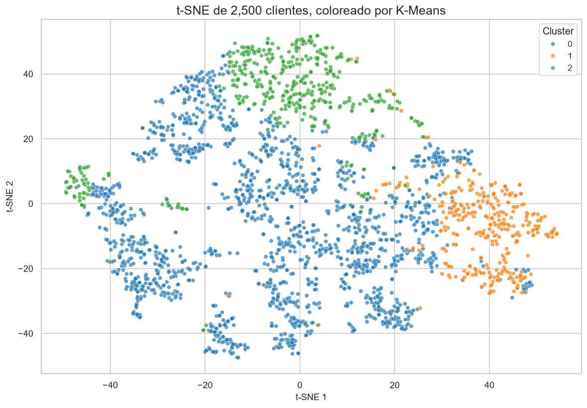
Figure 5. A stratified sample of the final K-Means labels shown in a t-SNE projection for visual inspection.

The projection shows structure and overlap but is not the fitting space. On the common comparison sample, K-Means records silhouette 0.251, Calinski-Harabasz 526.01 and Davies-Bouldin 1.58, the best combination among the three exhaustive baseline algorithms tested.

Customer profiles

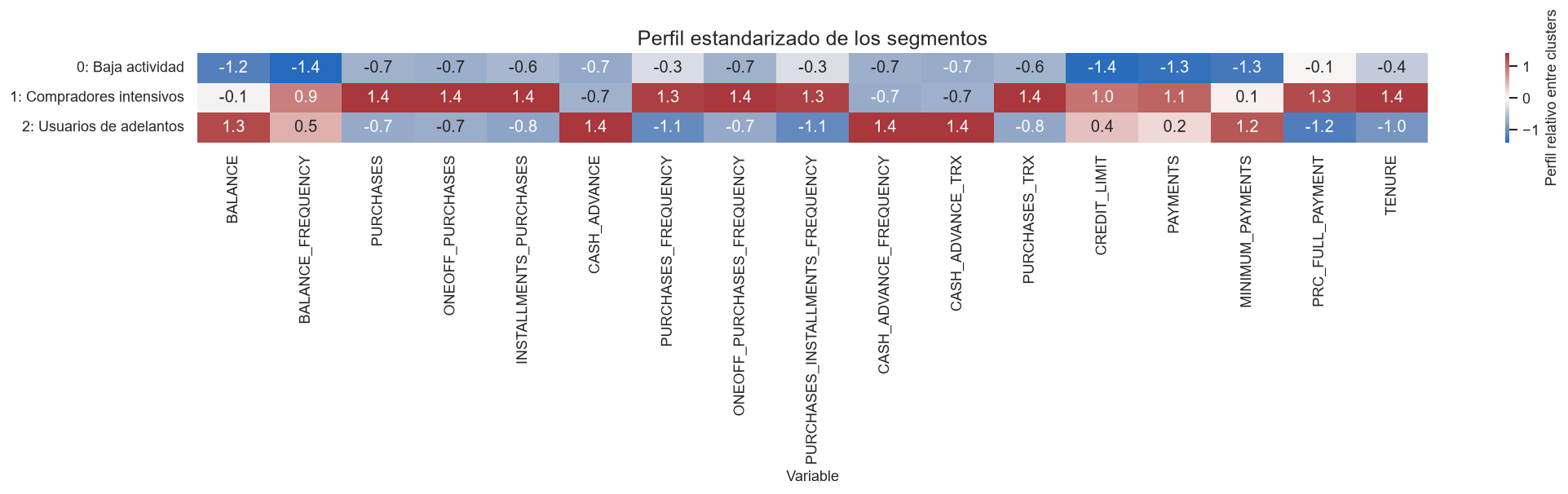
Figure 6. Segment means standardized relative to the full-dataset mean; the table below restores selected values to original units.

The executed profile table supports descriptive—not permanent—names:

Segment	Evidence in the original variables	Practical interpretation
Low activity	Mean balance 799.75; purchases 505.53; cash advance 330.82	Broad group with comparatively low account activity
Intensive purchasers	Purchases 4,268.52; purchase frequency 0.95; credit limit 7,733.97; payments 4,151.28	Frequent, high-value purchase behaviour
Cash-advance users	Balance 3,989.14; cash advance 3,866.21; full-payment rate 0.03	High balance and cash-advance use with low full-payment frequency

These averages make the clusters interpretable, but operational use would still require profitability, arrears and fairness evidence that the dataset does not contain.

Hierarchical clustering

Agglomerative clustering is inspected through a dendrogram built on a sample, then evaluated with three clusters on the same comparison sample used for the other exhaustive algorithms.

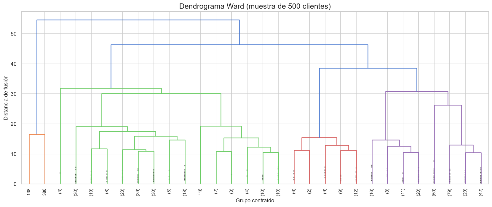
Figure 7. Ward-linkage dendrogram on a sample, used to inspect merging structure without rendering all 8,950 leaves.

Its silhouette is 0.17, Calinski-Harabasz 401.83 and Davies-Bouldin 1.81. It provides a useful structural comparison but separates the tested sample less clearly than baseline K-Means.

DBSCAN

DBSCAN is applied to the PCA(2) projection as an exploratory density analysis, not as the final customer segmentation.

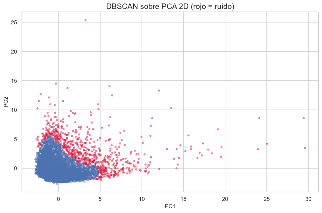
Figure 8. DBSCAN finds one main dense region and marks 681 customers as noise in PCA space.

The model identifies one cluster and 681 noise observations (7.6%). This configuration does not yield a useful exhaustive segmentation; its noise label means low density under the chosen representation and parameters, not fraud or business anomaly.

Algorithm comparison

Algorithm	Clusters	Silhouette	Calinski-Harabasz	Davies-Bouldin	Notes
K-Means	3	0.251	526.01	1.58	Best baseline metric combination
Agglomerative	3	0.17	401.83	1.81	Similar exhaustive objective
Gaussian Mixture	3	0.11	298.82	2.62	Soft probabilistic model, evaluated as hard labels
DBSCAN on PCA(2)	1 + noise	—	—	—	681 noise points; not an exhaustive segmentation

No single internal metric establishes business usefulness. The comparison supports K-Means as the clearest baseline only when its stronger internal metrics are considered together with the interpretable original-unit profiles.

Anomaly detection

Isolation Forest ranks unusual combinations of all standardized behaviours. The contamination value is explicitly set to 3% as an analytical assumption; it is not an estimate of fraud prevalence.

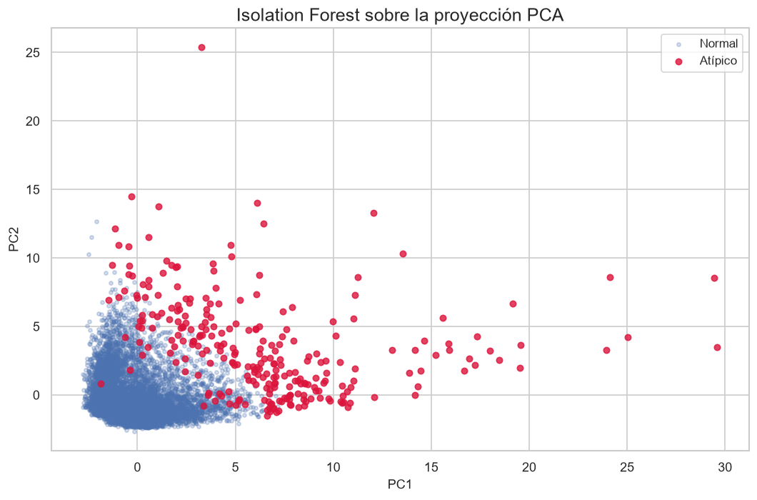
Figure 9. The model flags 269 observations for review and displays them on the PCA projection.

The flagged 269 customers are candidates for contextual review. The model does not establish fraud, error or customer value.

Advanced extension

The advanced notebook adds four derived indicators—credit utilization, average purchase per transaction, average cash advance per transaction and the payment-to-minimum ratio—then compares three representations.

Representation	Silhouette	Davies-Bouldin	ARI vs baseline	Largest cluster
Base	0.251	1.585	1.000	68.369%
Base + KPIs	0.175	1.796	0.392	54.749%
Base + KPIs + log1p	0.210	1.768	0.136	35.374%

Feature enrichment materially changes the segmentation. The KPI-plus-log1p version is more balanced but agrees weakly with the baseline and does not improve its silhouette; balance alone therefore does not make it a replacement.

Ten sub-sampling runs compare the advanced K-Means labels with the full-data reference solution. Their mean ARI is 0.933 ± 0.107, evidence of strong but not perfect stability under this resampling procedure.

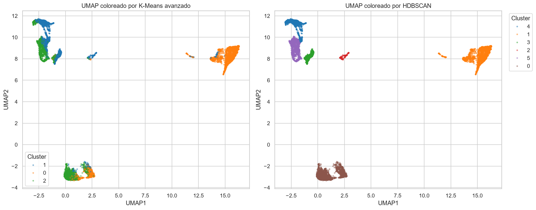
Figure 10. The same UMAP representation coloured by advanced K-Means and HDBSCAN assignments.

UMAP/HDBSCAN finds 6 clusters, 0% noise, and silhouette 0.727 within the UMAP embedding. Its ARI against advanced K-Means is 0.347, so the high embedding-space separation describes an alternative representation rather than automatic confirmation of the K-Means solution.

Key analysis indicators

Indicator	Value
Customers analysed	8,950
Baseline variables	17
Selected baseline k	3
Components retaining at least 80% PCA variance	7
Variance retained by those components	80.75%
Baseline K-Means silhouette	0.251
Baseline K-Means Calinski-Harabasz	526.01
Baseline K-Means Davies-Bouldin	1.58
Largest baseline segment	68.37%
Advanced sub-sampling stability ARI	0.933 ± 0.107

Conclusions

The baseline analysis finds three understandable behavioural profiles: a large low-activity group, intensive purchasers and customers characterised by high cash-advance use. Median imputation preserved all observations, and scaling was essential to stop monetary ranges from dominating distance-based models. K-Means provided the strongest tested baseline combination of internal metrics and interpretability.

The advanced representation changed cluster balance and membership substantially. Its sub-sampling stability was strong, while UMAP/HDBSCAN exposed a different six-cluster geometry rather than validating the same partition. Isolation Forest contributes a review queue for unusual behaviour but no fraud claim.

These results remain segmentation hypotheses, not ground truth. A genuine temporal validation cannot be performed because the available dataset contains six-month aggregates but no suitable date or repeated-period observations.

The full evidence is reproducible in workshop-clustering-creditcard.ipynb and workshop-clustering-creditcard-advanced.ipynb.